First steps on analyzing and stationarizing of time series data
A while ago I had the opportunity to work on building a sales forecaster as a POC. It was a challenging project with a cool MVP as an outcome. Through this post, I will share part of my journey and findings on analyzing the data I was provided.
Assumptions
I will assume you have previous knowledge of both Python and Pandas.
First things first…
This project started like every other data science project: familiarizing ourselves with the data we had in hand. I did this by importing the CSV file provided as a data source.

Once I had a clear idea of what kind of data we were dealing with, I proceeded with the initial exploration and usual transformations.

To simplify future manipulations over Pandas DataFrame, I made ‘fecha’ the index of the DataFrame. Since the records already came in the correct order, it was simple to perform this transformation and convert the DataFrame into a series with a ‘daily-level’ frequency, by resampling the entire DataFrame.


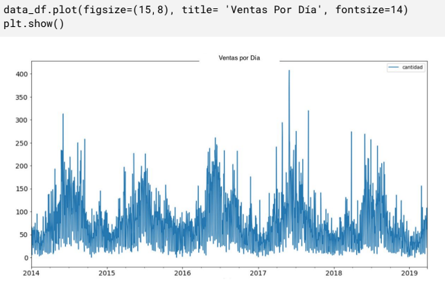
After completing the above transformations, the data was ready to be plotted. With the help of the Matplotlib library, I was able to display a graph of the quantity of product sold per day throughout the years.

So…what’s a time series and what makes it special?
From the initial data exploration, it was clear we were dealing with what is known as a time series. Time series is just a fancy way of saying we are dealing with data points indexed in time order.
Usually, when dealing with time series, we look for some special characteristics in our data to be able to make predictions based on it. Specifically, we look for a time series that is stationary.
Stationarity of a time series
We can say that a time series is stationary when its mean and variance are not a function of time (i.e. they are constant through time).
Stationarity is important because most of the statistical methods to perform analysis and forecasting work on the assumption that the statistical properties (mean, variance, correlation, etc.) of the series are constant in time.
How to test the stationarity of a time series?
Stationarity can be assessed in two ways:
● Visually inspect the data points and check how the statistical properties vary in time
● Perform a Dickey-Fuller test
Let us take a visual approach first and see how it goes:

By plotting the standard deviation and mean along with the original data points, we can see that both of them are somewhat constant in time. However, they seem to follow a cyclical behavior.
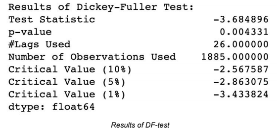
Although the visual approach can give us a clue, applying the Dicky-Fuller Test (DF-test) can provide a more precise way to measure the stationarity of our series.

I will not go through much detail on how the DF-test work, but let’s say all we need to care about is the numbers we see in “Test Statistic” and “Critical Values”. We always want the former to be less than the latter. And the lesser the value of Test Statistic the better.
Our series is stationary given that Test Statistic is less than all the Critical Values, though not by much.
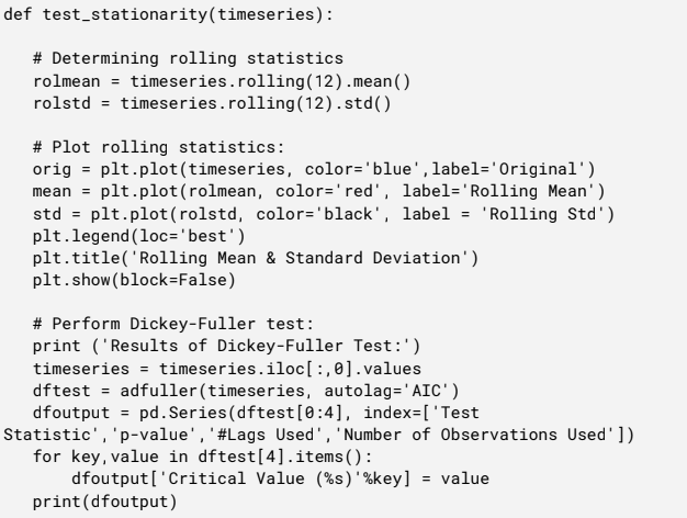
Below you can see the code I used to evaluate the stationarity:

What if our time series was non-stationary?
There are some techniques one can apply to stationaries a time series. The two I am more familiar with are:
● Transformation: apply transformation which penalizes higher values more than smaller values. These can be taking a log, square root, cube root, etc. This method helps in reducing the trend.
● Differencing: take the difference of the observation at a particular instant with that at the previous point in time. This deals with both trend and seasonality, hence improving stationarity.
Pandas and NumPy provide you with very practical ways to apply these techniques.
For the sake of demonstration, I will apply a log transformation to the DataFrame.

Bonus track: We can even apply a smoothing technique over the transformed data set to remove the noise that may be present. A common smoothing technique is to subtract the Moving Average from the data set. This can be achieved as easy as:

Clearly, we can see that applying log transformation + moving average smoothing to our original series resulted in a better series; in terms of stationarity.
To apply differencing, Pandas shift() function can be used. In this case, first-order differencing was applied using the following code.

Let us perform a DF-test on this new resulting series.

With the log transformation and differencing the test statistic is significantly smaller than the critical values, therefore this series is too more stationary than the original series.
Wrapping up…
When we face a predictive task that involves a time series, we need to analyze said series and determine whether it is stationary or not. To determine the stationarity, we can either plot the data and visually inspect the mean and other statistical properties or perform a Dickey-Fuller Test and look at the Test Statistic and Critical Values. In case the series happens to be non-stationary, we can apply techniques such as transformation or differencing to stationarize the series.
After all this analysis and preparation, the next step in the project was to forecast with the time series, but that’s a topic for another post!
Learn more from our team here, or check out our custom development services


1 Comment
Comments are closed.